Authors and guest post by Kamil Kovar
This is the second in a series of blog posts (the first can be found here) that present a new EViews add-in, SpecEval, aimed at facilitating development of time series models used for forecasting. This blog post will focus on the illustration of the basic outputs of the add-in by following a simple application, which will also illustrate the model development process that the add-in aims to facilitate. Next section provides brief discussion of this process, while the following section discusses the data and models considered. The main content of this blog post is contained in next two sections, which discuss basic execution before presenting the actual application.
Table of Contents
- Model Development Process
- Data and Models
- Execution
- Model Forecasting Performance
- Model Sensitivity
- Concluding Remarks
- Footnotes
Model Development Process
The SpecEval add-in was created with a particular model development process in mind. Specifically, the add-in is based on the belief that model development process should be both iterative and – more importantly – interactive. It should be iterative in that it proceeds in steps, each improving the earlier version of the model, be it in form of inclusion of additional regressors or modification of already included regressors. It should be interactive in that the improvements should be based on information about shortcomings of the earlier model. Importantly, this means that the development process should be done by human developer, rather than rely on computer algorithm, since it requires a modicum of imagination.
The workflow of the model development process is shown in figure below. The process starts with initial proposed model, which is then evaluated using the outputs of the add-in. These outputs contain multiple relevant pieces of information, from basic model properties entailed in estimation output such as regression coefficients, to forecast performance and finally sensitivity properties. Each of these can be used to identify shortcomings of the current model and propose modifications which will address these shortcomings, in an interactive model development process on part of model developer.

|
|
Figure 1: Model Development Process
|
Since in most situations the information can be ordered in terms of importance – e.g. "correct" coefficient signs are necessary, while desired degree of sensitivity often is not - one can view the process as linear, proceeding from basic properties through forecasting performance to sensitivity. We will roughly follow this model development process in the remainder of this blog post.
Data and Models
The add-in will be illustrated on modelling a relatively simple time series – an industrial production in Czechia.1 The quarterly series is displayed in figure below. It is clear, that the series is trending, but that it does not follow a deterministic trend. Correspondingly, in what follows we will use log-difference of industrial production as the dependent variable.

|
|
Figure 2: Czechia Industrial Production
|
What model should we use for forecasting industrial production? The answer to this question depends on the environment in which one is forecasting given series. The type of models can vary from simple univariate reduced from ARIMA models, through their multivariate multiequation cousins, VAR models, to structural single or multiple-equation models. Here we will illustrate the SpecEval add-in on the multivariate single-equation models for which the add-in is most suitable. The choice corresponds to environment where one has available forecasts for multiple potential right-hand side variables, such as GDP, and wants to “expand” these forecasts to industrial production, i.e. produce forecasts industrial production that are consistent with forecasts for other macroeconomic variables. This is fairly common task, especially in the context of macroeconomic stress testing.
Within this class of models, our starting point is simple regression linking a log-difference of the industrial production to a log-difference of the GDP:
$$
\text{dlog}(IP_{t}) = \beta_0 + \beta_1 \text{dlog}(GDP_t)
$$
This equation simply postulates that current growth rate of industrial production can be well predicted by the current growth rate of GDP, a reasonable postulation, given that both are measures of economic activity. Later we will enrich this model by including additional variables/regressors based on the analysis of this model. Before considering additional multivariate models, though, we will use simple ARIMA(0,1,2) model as our benchmark. The first equation is called EQ_GDP while the second is called EQ_ARIMA.
Execution
SpecEval allows modeler to produce a report by either executing it through GUI or issuing the relevant command from given equation object, an approach we take here:
eq_gdp.speceval(noprompt)
This command would produce and display spool with several output objects that can be used to evaluate the given equation (see left panel of figure below). However, it is more interesting to consider the given equation in context of the benchmark ARIMA equation and hence execute SpecEval for both equations, what can be don by simply adding another equation to a list of specifications:
eq_gdp.speceval(spec_list=eq_arima)
What we have done here is just specify that the list of specification for which the add-in will be executed should include also ‘eq_arima’ equation. As a result, the add-in will produce and display spool that is organized by the type of output, so that same outputs for different specifications are next to each other, facilitating quick comparison. See right panel of figure below.

|
|
Figure 3: Output Spools
|
Model Forecasting Performance
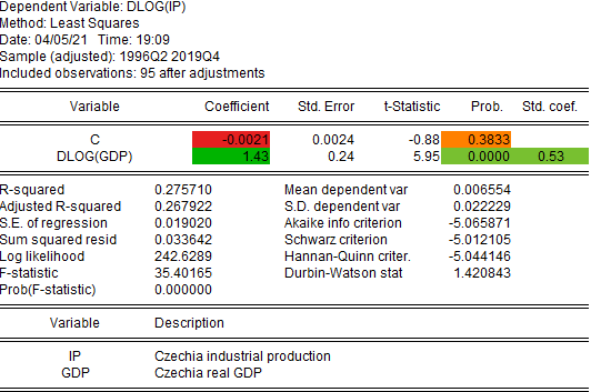
Starting point of analysis of any forecasting model is of course its estimation output, and so SpecEval includes it among its outputs. Rather than using the standard estimation output reported by Eviews, the SpecEval reports estimation output that is enhanced in several ways, such as color coding and formatting of numbers, as well as information about included variables:

|
|
Figure 4: Czechia Industrial Production - Estimation
|
Estimation output provides some basic information about the model. However, it provides limited information about forecasting performance. True, statistics like R-squared, standard deviation of residual, or Durbin-Watson statistic can be re-interpreted as indicators of forecasting performance, but only as very limited ones. Addressing this shortcoming is one of the key motivations for SpecEval and hence the report includes explicit information about forecasting performance.
First, there is table with values of forecast precision metrics, such as Root Mean Square Percentage Error (RMSPE), that are color-coded according to their rank. For our application this table shows that the proposed model is worse in terms of forecasting performance than the benchmark ARIMA model if we consider longer forecasting horizons, which is dispiriting conclusion given that our model includes additional information.

|
|
Figure 5: Czechia Industrial Production - RMSPE
|
Before despairing and concluding that GDP is not useful for forecasting industrial production, it is useful to look at forecasting performance in more detail than what is incorporated in the summary statistics. Specifically, we can leverage the second output focused on forecasting performance, the forecast summary graphs. The motivation for those is simple: precision metrics are summary statistics over the whole backtesting sample, and hence it is possible that they mask important heterogeneity across the sample, something that forecast summary graphs will immediately reveal. This is indeed the case in our application since bad forecasting performance for the our model is concentrated in the early periods – after 2000 the forecasting performance looks much better than that of the benchmark model.

|
|
Figure 6: Czechia Industrial Production - Forecast Summary
|
SpecEval provides flexibility to explore this issue in further detail. For example, the forecasting performance in beginning of the sample is so bad that one would likely suspect issues with the estimated coefficients. To check this out, we can include coefficient stability graphs among the outputs:
eq_gdp.speceval(spec_list=eq_arima)
Here we just specified that the execution list should also include stability outputs, apart from the normal outputs. The resulting graph displayed below shows the full time series of recursive regression coefficients, together with their standard errors. What is crucial from our perspective, is that the graph indeed confirms our suspicions: the coefficient on GDP in the early parts of the sample is negative, which is at odds with our expectations and likely reflects the very small number of observations used for estimation in the beginning of the backtesting sample.

|
|
Figure 7: Czechia Industrial Production - Coefficient Stability
|
Another way we can explore this issue is to switch from out-of-sample to in-sample forecasting. In other words, we can use the actual equation estimated on the full available sample to make the individual backtest forecasts. Or alternatively, and more simply, we can stick with out-of-sample forecasts but limit the evaluation sample to start in 2000q1. The two execution commands corresponding to these options are following:
        eq_gdp.speceval(spec_list=eq_arima,oos=”f”)
        eq_gdp.speceval(spec_list=eq_arima,tfirst_test=”2000q1”)
Either of these approaches show that the initial superiority of ARIMA model was consequence of bad forecasts based on short estimation sample, as evidenced by tables below. Crucially, these early forecasts do not provide approximation of what the forecast would be at that point in time: any economist operating the model would likely discard forecasts from model with negative coefficient on GDP. However, without the knowledge of this artifact of the results – such as when we would rely on precision metrics alone, as is customary - we would potentially discard the model altogether. This shows both the value added by the SpecEval and its flexibility, and the value of incorporating graphical information about forecasting performance. Document ‘SpecEval illustrated’ provides many additional examples of this flexibility and how it can be leveraged in developing forecasting models.

|
|
Figure 8: Czechia Industrial Production - In-Sample RMSPE
|
Model Sensitivity
The second main focus on SpecEval outputs – in addition to forecasting performance – is evaluation of model sensitivity, that is how does the proposed model respond to outside shocks. There are three types of outputs that belong to this category. First, SpecEval allows user to specify set of historical sub-samples for which forecasts performance can be analyzed separately, be it in terms of forecast precision metrics or in terms of forecast graphs, on which we will focus here. The above figures captured the forecasting performance over the whole sample, but sometimes performance for particular historical period is of special interest given their unusual nature relative to the rest of the backtest sample. An example from credit risk modelling are recessionary periods or periods of financial stress. To analyze such period in context of our example, we simply need to include specify sub-samples of interest:
eq_gdp.speceval(subsamples=”2008q3-2009q4, 2011q3-2013q2”,oos=”f”)
The top panels of figure below show the resulting graphs which capture the forecast from our model over the period of Great Recession and European Sovereign Debt Crisis. The conclusion is not very positive since the model fails to predict the magnitude of the decline in industrial production, especially during the Great Recession.

|
|
Figure 9: Czechia Industrial Production - Subsample Forecast
|
One potential solution is to allow for the relationship between GDP and industrial production to be different during normal and recessionary periods by adding interaction with dummy variable indicating recessionary period:
$$
\text{dlog}(IP_{t}) = \beta_0 + \beta_1 \text{dlog}(GDP_t) + \beta_2 \text{dlog}(GDP_t) D_t^recession
$$
")
|
|
Figure 10: Czechia Industrial Production - Estimation (Recession)
|
The forecasts from resulting model captured in bottom panels of the above figure show significant improvement over the original model in terms of forecasting during recessionary periods in context of in-sample forecasting.
Second category of outputs focused on model sensitivity displays conditional scenario forecasts made using given model specification. This entails making forecast for the dependent variable under alternative scenario paths for the independent variables. While this is especially useful in situation when such scenario forecasting is of interest, it is useful more generally in model development as source of alternative information about the model and its behavior, something we illustrate here. To obtain conditional scenario forecasts using SpecEval we just need to specify list of scenarios as one of the arguments as in the first argument in following command:
eq_gdp_dummy.speceval(scenarios=”bl sd”,exec_list=”normal scenarios_individual”,tfirst_sgraph=”2006q1”, graph_add_scenarios="gdp[r],trans=”deviation”)
Here, apart from the list of scenarios, we have specified several other options: we have indicated that we want to have individual scenario graphs as the output (rather than graphs showing all scenarios together); that we want the scenario graphs to start in 2006q1; that they should also include GDP (as opposed to only the industrial production); and that the transformation charts should be in terms of deviations from baseline. Top panels of figure below show the graph capturing level of the forecast and graph capturing the deviation from baseline, respectively. These leave us with mixed feelings about the model. On the positive side, the decline in industrial production seems appropriate given the decline in GDP - as was historically the case, industrial production does fall significantly more than GDP, reflecting the fact that the combined coefficient is above 2. On the negative side the industrial production remains significantly below GDP even in the long run, which seems counterintuitive - one would expect both the drop and rebound in industrial production to be larger so that the permanent effect on industrial production is only slightly larger than for GDP.

|
|
Figure 11: Czechia Industrial Production - Forecast Scenario
|
The reason why the model fails to make such forecast is because it makes industrial production more sensitive movements in GDP only during recessions, not during recoveries. One simple way to address this is to replace the dummy indicating recession by dummy that captures both recessions and recoveries. Here, we simply use new dummy that is now equal to 1 also 4 quarters after the end of recessions:
$$
\text{dlog}(IP_{t}) = \beta_0 + \beta_1 \text{dlog}(GDP_t) + \beta_2 \text{dlog}(GDP_t) (\text{@}movav(D_t^recession, 4) > 1)
$$
The resulting scenario forecasts are in bottom panels of figure above and show that the model modification addressed our initial concerns: industrial production still falls more than GDP, but then also rebounds more strongly so that in the long run the shortfall in industrial production is only slightly larger than that of GDP.
The inclusion of recession dummy was motivated by shortcomings of the model in terms of historical forecasts during recessionary periods, while its replacement by recession-and-recovery dummy was motivated by shortcomings in terms of scenario forecasts. However, it turns out that both modifications also help a lot with overall forecasting performance, as evidenced in the table below. In this sense analysis of model sensitivity and especially of its behavior in conditional scenarios are complementary to analysis overall forecasting performance and hence useful for model development purposes even if model sensitivity and scenario forecasting is itself not of importance.
")
|
|
Figure 12: Czechia Industrial Production - In-Sample RMSPE (Scenario)
|
Final category of model sensitivity outputs is composed of shock response graphs. The concept should be familiar from the VAR literature: one studies how does the dependent variable respond to shocks to individual independent variables.2 SpecEval implements this procedure for single equation multivariate time series models; one simply needs to include shocks in the execution list:
eq_gdp_dummy2.speceval(exec_list=normal shocks, shock_type=transitory)
As a result, the report will now include two types of figures corresponding to two types of shocks, depending on whether the underlying independent variables or the actual regressor is being shocked. In either case the corresponding figure shows 4 graphs: (1) graph with two paths for the underlying dependent variable, without shock and one with shock, (2) graph with deviation/difference between the two paths, (3&4) analogical graphs for the shocked variable/regressors. Below is example for a modified version of our model with dummy variable, which now includes also lagged dependent variable and lag of the GDP regressor. This means that the model now belongs to the Autoregressive Distributed Lag (ARDL) family, making its shock responses dynamic and hence hard to gauge from estimation output alone. For such models visualizing the exact shock responses can be very valuable. For example, in current context the transitory decrease in GDP (see bottom panels) leads to initial drop in industrial production, which is then reversed so much that industrial production is above the no-shock path for several quarters (see top panels).

|
|
Figure 13: Czechia Industrial Production - Shock-Response
|
This shock response might be unappealing from scenario perspective because it can easily lead to downside scenarios characterized by recession and recovery in GDP featuring industrial production that temporarily rises above baseline. In this way studying shock responses can be important tool when models will be used in scenario forecasting. However, the value is not limited to this use case: the above shock response would probably alert the modeler that different model structure – for example replacing lagged dependent variable with autoregressive error – might be preferable from forecasting perspective. Indeed, while the ARDL model has worse forecasting performance than the model without any lagged components, model that includes only AR(1) error – and hence does not feature the shock response reversals - has significantly better forecasting performance, as shown in table below.

|
|
Figure 14: Czechia Industrial Production - RMSPE Comparison
|
Concluding Remarks
This part of the blog post series dedicated to SpecEval was focused on showcasing how SpecEval can be operated, what are the basic outputs and how they can be leveraged in model development process. However, for the sake of brevity the possibilities highlighted here were far from exhaustive – reader should consult ‘SpecEval illustrated’ document for more detailed discussion. That said, the next blog post in this series will focus on one particular functionality of SpecEval – the use and value of transformations in model development process.
Footnotes
1. The data and together with program that will replicate the outputs reported here can be found on my personal website.↩
2. This kind of analysis is readily available in Eviews (or other statistical packages) for VAR models. However, this type of analysis is puzzlingly uncommon in case of single equation multivariate time series models, and correspondingly is not supported by Eviews of other statistical packages, a gap SpecEval tries to fill. Note that for univariate ARIMA models Eviews – unlike most other statistical packages - does support this kind of analysis.↩
3. Note that these two features – in-sample forecasting and inclusion of multiple equations in the forecasting model – are possible thanks to in-built EViews functionality and hard to replicate in other statistical programs. The former is thanks to the separation between estimation and forecasting samples, the latter thanks to flexible model objects.↩


")

")


No comments:
Post a Comment