Friday, November 4, 2016

L1 Trend Filtering

Author and guest post by Eren Ocakverdi.


Extracting the trend of a time series is an important analytical task as it simply depicts the underlying movement of the variable of interest. Had this so-called long term component known in advance, we would have been able to foresee its future course. In practice, however, there are several other factors (e.g. cycle, noise) in play that have influence on the dynamics of a time dependent variable.

Time path of a variable can either be deterministic (assuming the change in trend is constant) or stochastic (assuming the change in trend varies randomly around a constant). Estimation of a deterministic trend is straightforward, yet it often oversimplifies the data generating process. The assumption of stochastic trend seems to be a better fit to observed behavior of various time series as they tend to evolve with abrupt changes. Nevertheless, its estimation is difficult and can have serious implications due to accumulation of past errors.

Tuesday, October 18, 2016

Add-in Round Up for 2016 Q2/Q3

Add-in Round Up for 2016 Q2/3

In this section of the blog, we provide a summary of the Add-ins that have been released or updated within the previous few months, and we announce the winner of our “Add-in of the Quarter” prize!

As a reminder, EViews Add-ins are additions to the EViews interface or command language written by our users or the EViews Development Team and released to the public. You can install Add-ins to your EViews by using the Add-ins menu from within EViews, or by visiting our Add-ins webpage.

We have 9 new Add-ins within the last few months, including a number related to VAR analysis: 
  1. ThSVAR
  2. FanChart
  3. Croston
  4. LocalIRFs
  5. Speccaus
  6. SIRF
  7. ConfCast
  8. URAll
  9. DMA

ThSVAR

The ThSVAR Add-in continues Davaajargal Luvsannyam's line of VAR based Add-ins, and estimates Threshold Structural Vector Auto Regression (FAVAR) models, such as those described by Balke (2000).

Unlike traditional structural VAR approaches, the ThSVAR allows a threshold variable that determines which of two regimes the structural contemporaneous relationship is in.

FanChart

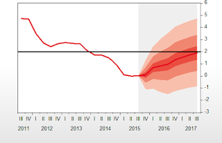
The FanChart add-in creates Bank of England style fan charts from forecast distribution data.  More details can be found on our Fan Chart blog post.

Croston

The Croston method is a way of using exponential smoothing techniques to forecast intermittent series (series with long periods of zeros, intermingled with sparse positive integers).  This add-in performs the Croston method in a simple fashion.

LocalIRFs

The LocalIRFs Add-in, written by Eren Ocakverdi (Trubador on the EViews forums), performs impulse response analysis by local projection method of Jordà (2005, 2009) on a previously estimated VAR model. 

As well as providing the impulse response graphs and tables, Eren allows equality hypothesis tests on the responses.

Speccaus

Nicolas Ronderos' speccaus Add-in computes a frequency domain Granger causality test in the context of VAR models, as given in Breitung and Candelon (2006). 

SIRF

Another Davaajargal Luvsannyam Add-in related to VARs, SIRF computes scaled impulse responses of Structural Vector Auto Regressions. 

Although a rather simple Add-in, it provides powerful functionality to users who wish to create their own impulses for structural VARs.

ConfCast

One more from Davaajargal Luvsannyam (who has been busy!) to add to the extensive list of VAR based add-ins.  ConfCast performs conditional forecasting from a VAR model, allowing you to constrain the future values of the VAR's underlying series.

URALL

URALL, by Imadeddin Almosabbeh, solves a time-old issue of wanting to perform individual unit root tests on a large number of series at once.  The add-in allows you to specify the type of unit root test to run, then collates the output from each one into an easy to read table. Nifty!

DMA

The final Davaajargal Luvsannyam add-in, and one unrelated to VARs!, performs dynamic model averaging.  

Model averaging is an exploding field in econometrics, with a common consensus held that averaging over different models is a better approach than choosing the single best model. 

Although EViews (9 and above) has various model averaging techniques built, dynamic model averaging is not yet available built in.  This add-in addresses that short-coming.


Quarterly Prize

The EViews Development Team has decided that the DMA Add-in contributed most significantly to the usage of EViews this quarter. 
For more information on writing Add-ins, you can read the Add-in chapter of the online help or visit the Add-in writer’s forum

If you would like to submit an Add-in, need more information on the Quarterly Prize, or have quesitons about writing Add-in for EViews, please email support@eviews.com.

Tuesday, August 9, 2016

An Application of Data Filtering Extracting Super Cycles in Commodity Prices

Authors and guest post by Daniel L. Jerrett, Ph.D and Abdel M. Zellou, Ph.D.

EViews offers numerous techniques to filter time series including the Hodrick Prescott filter as well as various band-pass filters.

This article will describe an application of one of these filtering techniques, namely the asymmetric Christiano Fitzgerald band pass filter, and its applications to real oil prices in order to extract the various cycle and trend components.

Super Cycles and Christiano Fitzgerald Band Pass Filter

There is a long standing interest in commodity price dynamics, i.e. their trend, cycle and volatility (Cuddington et al. 2007, Cashin and McDermott 2002). Recently, a number of papers have focused on the super cycle hypothesis. A super cycle (SC) is “a prolonged (decades) long trend rise in real commodity prices. Heap (2005) and Cuddington and Jerrett (2008) define a super cycle as a cycle lasting 20 to 70 years (trough to trough) as an economy goes through structural transformation caused by industrialization and urbanization. This structural transformation is accompanied by increased demand for energy and metals commodities as the manufacturing sector expands. Historically, these periods of urbanization and industrialization have occurred in Europe during the Industrial Revolution in the 19th century, in the U.S. at the beginning of the 20th century, in Western Europe again during the reconstruction that followed the Second World War, in South-East Asia in the 1960s and finally in the BRIC1 countries in the 1990s2. The increase in demand for energy and metals commodities during these periods, combined with the delay for the supply to catch up with the demand surge, created sustained periods of high commodity prices according to the super-cycle hypothesis.

Wednesday, July 13, 2016

All About Excel

Microsoft Excel is still used by many users and this post will quickly go over all of the different ways you can share and move data between EViews and Excel.

Native Excel File Support

EViews offers direct Excel file read and write capability. If you have data in an existing Excel spreadsheet and you wish to use it in an EViews workfile, simply drag and drop the Excel file onto an EViews workfile to start the import (see IMPORT command and Importing Data in our User's Guide) or drop it onto an empty area in the EViews frame window to create a new workfile (see WFOPEN command).


At the end of the import, you also have the option to link the data back to the source spreadsheet. This will allow you to easily refresh the data in the workfile, whenever the source Excel data has changed (see WFREFRESH).

By default, EViews will try to read in objects by column and will look for a single header row for the object names. In addition, EViews can transpose the data before import if your objects are defined in rows instead.

In the other direction, you can save EViews workfiles directly to an Excel file by going to
File –> Save As, then selecting the proper Excel type in the Save as type dropdown (see WFSAVE command and Exporting Data in our User's Guide).

Note: Reading the newer Excel .XLSX file format was added in EViews 7. Saving in .XLSX format was added in EViews 8.

Thursday, June 23, 2016

Impulse Responses by Local Projections


Author and guest post by Eren Ocakverdi.


Vector Autoregression (VAR) is a standard tool for analyzing interactions among variables and making inferences about the historical evolution of a system (e.g., an economy). When doing so, however, interpreting the estimated coefficients of the model is generally neither an easy or useful task due to complicated dynamics of VARs. As Stock and Watson (2001) aptly puts it, impulse responses are reported as a more informative statistic instead.

The Impulse Response Function (IRF) measures the reaction of the system to a shock of interest. Unfortunately, when the underlying data generating process (DGP) cannot be well approximated by a VAR(p) process, IRFs derived from the model will be biased and misleading. Jordà (2005) introduced an alternative method for computing IRFs based on local projections that do not require specification and estimation of the unknown true multivariate dynamic system itself1.

The usual presentation of IRFs is through visualizing the dynamic propagation mechanism accompanied by error bands. In addition to marginal error bands, Jordà (2009) introduced two new sets of bands to represent uncertainty about the shape of the impulse response and to examine the individual significance of coefficients in a given trajectory. In this framework, it becomes straightforward to impose restrictions on impulse response trajectories and formally test their significance.

Wednesday, April 27, 2016

Fan Chart

Fan charts are a method of visualizing a distribution of economic forecasts, pioneered by the Bank of England for their quarterly inflation forecasts.

We are often asked if EViews can produce fan charts. At its heart, a fan chart is simply a type of area band chart. EViews has been able to produce area band charts for a number of previous versions. So whenever we have been asked if EViews can produce fan charts, we have said “yes”.

Recently, we decided to go one step further and replicate an official Bank of England fan chart in EViews, and this blog post will document the steps required to perform the replication.

We have decided to replicate a recent inflation report fan chart, specifically the November 2015 inflation fan chart available from the Bank of England.

Tuesday, April 5, 2016

Add-in Round Up for 2016 Q1

In this section of the blog, we provide a summary of the Add-ins that have been released or updated within the previous few months, and we announce the winner of our “Add-in of the Quarter” prize!

As a reminder, EViews Add-ins are additions to the EViews interface or command language written by our users or the EViews Development Team and released to the public. You can install Add-ins to your EViews by using the Add-ins menu from within EViews, or by visiting our Add-ins webpage.

We have five new Add-ins within the last few months:
  1. BFAVAR
  2. SRVAR
  3. TVSVAR
  4. FORCOMB
  5. TSCVAL

BFAVAR

The BFAVAR Add-in, written by Davaajargal Luvsannyam, estimates Factor Augmented Vector Auto Regression (FAVAR) models using the one-step Bayesian likelihood approach.

Wednesday, March 23, 2016

pyeviews: Python + EViews


Since we love Python (who doesn’t?), we’ve had it in the back of our minds for a while now that we should find a way to make it easier for EViews and Python to talk to each other, so Python programmers can use the econometric engine of EViews directly from Python. So we did! We’ve written a Python package called pyeviews that uses COM to transfer data between Python and EViews (For more information on COM and EViews, take a look at our whitepaper on the subject).

Here’s a simple example going from Python to EViews. We’re going to use the popular Chow-Lin interpolation routine in EViews using data created in Python. Chow-Lin interpolation is a regression-based technique to transform low-frequency data (in our example, annual) into higher-frequency data (in our example, quarterly). It has the ability to use a higher-frequency series as a pattern for the interpolated series to follow. The quarterly interpolated series is chosen to match the annual benchmark series in one of four ways: first (the first quarter value of the interpolated series matches the annual series), last (same, but for the fourth quarter value), sum (the sum of the first through fourth quarters matches the annual series), and average (the average of the first through fourth quarters matches the annual series).

Friday, March 18, 2016

How We Decide Which Features To Add


As developers of econometric software, one of the most common questions we are asked is how we decide which features to add to the next release of EViews.

There isn’t an easy way to answer this question – the process is often fluid and is different for every feature. Feature ideas generally come to us from one of the following sources:
·
  • Directly from our user base, either on the EViews forum, through our technical support channels or through face to face meetings. 
  • From reading journal articles and text books to discover the latest trends in the field.
  • From visiting academic and professional conferences, such as ASSA, NABE or ISF.
  • From meetings held at our user conferences.
  • Research from our development team.

The recent release of EViews 9.5 gives us a chance to explore the process with some examples.

MIDAS

Perhaps the most anticipated feature in EViews 9.5 is MIDAS estimation, which allows estimation of regression models using data of different frequencies. MIDAS first came to our attention a few years ago during a casual conversation between our developers and one of our academic users at the Joint Statistical Meetings.

Our user suggested that EViews’ natural handling of data from different frequencies and our emphasis on time series analysis, coupled with MIDAS’ growing popularity made it a great candidate for a new feature.

Following up on that discussion, our development team began researching what would be involved in adding MIDAS to EViews. MIDAS would be the first estimation technique in EViews that inherently uses data based on different workfile pages.

While later attending the EViews co-sponsored ISF conference, we also noticed that a large part of the conference was devoted to MIDAS estimation and forecasting as well as nowcasting. By this time we were convinced that MIDAS was an obvious choice to add to EViews.

Friday, February 12, 2016

Rolling Regression

Rolling approaches (also known as rolling regression, recursive regression or reverse recursive regression) are often used in time series analysis to assess the stability of the model parameters with respect to time.

A common assumption of time series analysis is that the model parameters are time-invariant. However, as the economic environment often changes, it may be reasonable to examine whether the model parameters are also constant over time. One technique to assess the constancy of the model parameters is to compute the parameter estimates over a rolling window with a fixed sample size through the entire sample. If the parameters are truly constant over the entire sample, then the rolling estimates over the rolling windows will not change much. If the parameters change at some point in the sample, then the rolling estimates will show how the estimates have changed over time.

Thursday, January 14, 2016

Object Linking and Embedding (OLE)

EViews has many users whose workflow includes repeatedly copying and pasting graphs and tables from EViews into the same Microsoft Office documents every time data or results are updated. We also have users who would like to give their colleagues the ability to adjust the appearance of their graphs and/or tables but without having the source workfile. One possible solution for both sets of users is to use Object Linking and Embedding (OLE).

Object Linking 

Object linking allows you to place your EViews graph or table into a Microsoft document but maintain a link/connection to the series or object in your EViews workfile. When changes are made to the source EViews workfile, those changes can be reflected immediately in the objects within the Microsoft document.